

Blog
Modelling dike breaching using TELEMAC-2D - A December 2013 case study
Monday, 16th January 2017
This blog was first published as a Linkedin article (see here) but is republished here.
On December 5th-6th 2013, Cyclone Xaver generated storm surge levels along the coastal regions of the southern North Sea that were the highest on record at some tide gauge locations on the UK East Coast, exceeding those of the disastrous 1953 event. However, this time the UK was better protected by coastal defences and flood warnings gave people more time to be prepared. At the time I was working at Risk Management Solutions and we went to visit some of the sites affected by the surge to survey the damage. We found that the defences had generally performed well and had prevented more serious flooding (more info here). However, it was apparent that in some cases the existing defences had only just prevented serious flooding for an event of this magnitude or were breached, causing flooding.
In Boston, Lincolnshire, the River Haven burst its banks as the storm surge propagated up the estuary flooding many homes, businesses and the historic church. Just outside Boston dike failure led to the inundation of a waste recycling plant, a number of warehouses, business units and the surrounding crop fields. The site and approximate breach location (shown in red) can be seen in the image below.
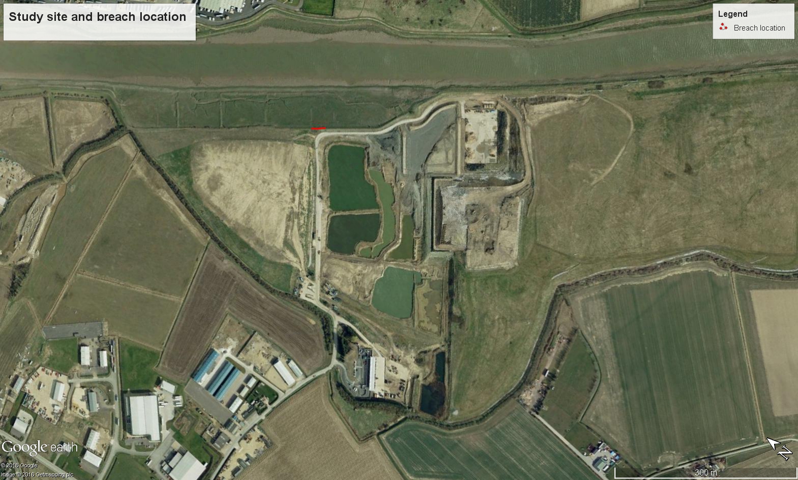
Predicting breaches, such as this one, is hard to do as they often occur due to very specific local water levels and/or wave conditions and differences in the dike level or structural integrity. However, it may be useful to model breaching scenarios at various locations to investigate the potential impact and make more informed decisions on allocating resources to defence construction and maintenance.
TELEMAC-2D allows you to simulate dike breaching for a range of scenarios and breach growth mechanisms. Data such as the Spatial Flood Defences dataset and LIDAR digital surface models at 1 m resolution are now publicly available and allow you to identify defence assets that could be liable to breaching and resolve features such as dikes in hydrodynamic simulations.
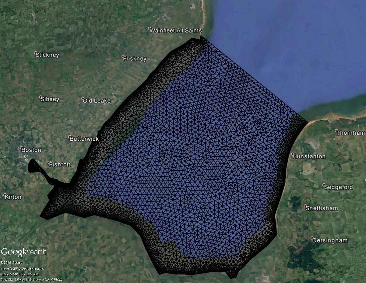
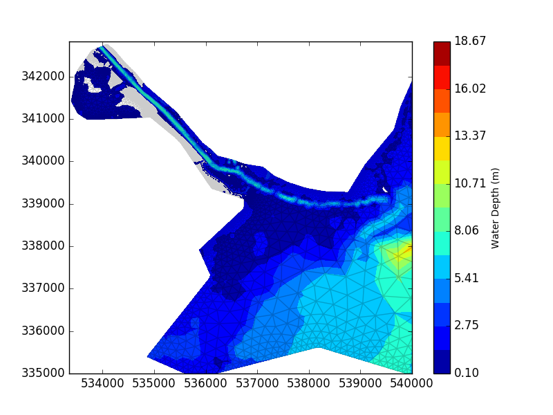
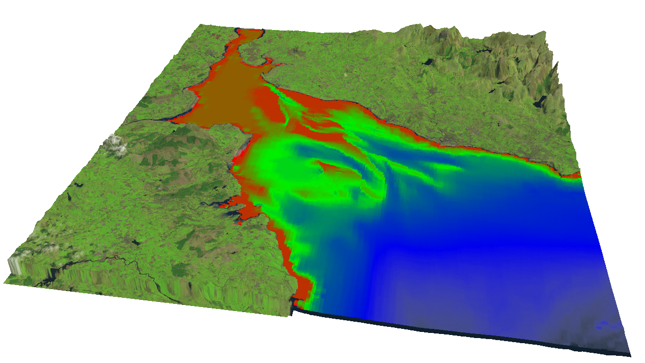
To simulate the dike breach at the recycling plant near Boston in December 2013, a mesh was created in Blue Kenue using publicly available data. The mesh extends offshore from the study site to simulate the surge propagation into the region resolving the River Haven and region of inundation at increased resolution.
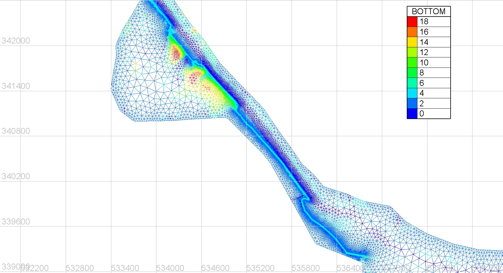
The 1 m LIDAR data and high density of mesh elements allows the dike to be well resolved and can be seen in light blue in the image below.
This event can be accurately simulated based on knowledge of the breach location and the approximate region of inundation and visualized in 3D using Blue Kenue (see below). The method can be extended to simulate other such historic events or breach scenarios and is a useful tool for investigating the impacts of dike breaching. However, simulating multiple events/breach scenarios is computationally expensive due to the small time-step and element size needed to resolve dikes in the hydrodynamic simulation, but could be partially resolved through the use of CPU clusters and parallel processing.
Visualising uncertainty in coastal flood predictions
Wednesday, 1st February 2017
Predicting coastal flooding at a particular return period has a degree of uncertainty associated with it. Some of the uncertainty may be safely ignored and will make little difference to the final simulated flood footprint. However, some of the uncertainty lies in such a range that it can make a significant difference to the predicted flood extent and cannot be ignored when considering the possible consequences for a given return level. Some sources of uncertainty in coastal flood modelling include:
- The surge level at the coast
- The height/strength of the defences
- The DTM and the interpolation method if reinterpolated
- The roughness coefficient possibly derived from land use land cover data
- The overtopping volume due to waves
At longer return periods the uncertainty increases and becomes harder to quantify, as does the consequence this uncertainty poses. Another challenge resides in relating this uncertainty in a meaningful way to decision/policy makers that may have implications for coastal planning. If the uncertainty in the 100 year return period surge level is +/- 0.4 metres, what does that really mean or look like for a given location?
This blog post aims to visualise the range in the predicted flood extent due to the most significant sources of uncertainty, focusing on Hornsea on the UK East Coast. Hornsea has suffered from significant coastal erosion where sand transported by longshore drift (read more here), and subsequent cliff erosion, has lead to a need to manage the region's natural defences to wave attack and flooding. Hornsea has also been flooded twice in recent times when storm surge and waves have overtopped the town's coastal defences. Significant flooding occurred in December 2013 and more recently on January 13th 2017, where predicted storm surge levels lead to an evacuation of part of the town as homes and businesses suffered flooding. Hornsea is susceptible to coastal flooding by surge and wave levels that exceed the coastal defence elevation as it has a region of low-lying land (seen here) where flood warnings are issued by the Environment Agency. The Environment Agency also publish extreme sea levels in a coastal design sea levels database (about to be updated) derived from extreme value analysis, joint probability and numerical modelling. The database includes a range of uncertainty based on the methods used to derive each return period sea level.
In the following example the flood footprint is simulated (using flood modeller) at Hornsea due to the range of uncertainty in the 100 year return period coastal water elevation and the overtopping due to 3 m waves at the defences. The wave overtopping is dependent on the water level that determines the freeboard at the defences. The range of uncertainty for the 100 year return period water level at Hornsea is +/- 0.4 m. The range of uncertainty in the overtopping volume for the given wave condition can be examined by subtracting or adding one standard deviation to the coefficients in the equations that determine the mean overtopping discharge in the Eurotop manual. The manual recommends that you should increase overtopping discharge by one standard deviation from the mean for determining design heights as a safety measure. The default footprint (Simulation 0) is determined by the mean 100 year return period water level and the mean overtopping discharge. The other footprints are determined by combining the different uncertainties and are summarised in the following table.
| Surge (m) | Wave overtopping, Q (m^3/s) | Flooded area (m^2) | % change | |
|---|---|---|---|---|
| Sim 0 | +/- 0 | Mean | 149550 | 0 |
| Sim 1 | -0.4 | -1 Std dev | 63100 | -58 |
| Sim 2 | -0.4 | Mean | 98550 | -34 |
| Sim 3 | +/- 0 | -1 Std dev | 103375 | -31 |
| Sim 4 | +/- 0 | +1 Std dev | 206450 | +38 |
| Sim 5 | +0.4 | Mean | 254325 | +71 |
| Sim 6 | +0.4 | +1 Std dev | 271875 | +82 |
The bar chart below shows the percentage change in flooded area from the default for each simulation. Click on the bars to see the resultant flood footprint for each simulation or click on the image area to go back to the default.
Visualising the simulated flood footprint in the range of some of the uncertainties shows that there is a significant variation in its extent. This uncertainty should be taken into consideration when planning coastal flood protection schemes. Whilst it would be ideal to protect against the worst case scenario for a given return period, cost and aesthetics are likely to result in a compromise. Coastal flood modelling is a useful tool to examine the range of uncertainty, its consequences and to aid the planning of coastal flood protection measures so that critical infrastructure is safeguarded. Read more here.
Infrastucture and flooding: an impact study
Friday, 3rd March 2017
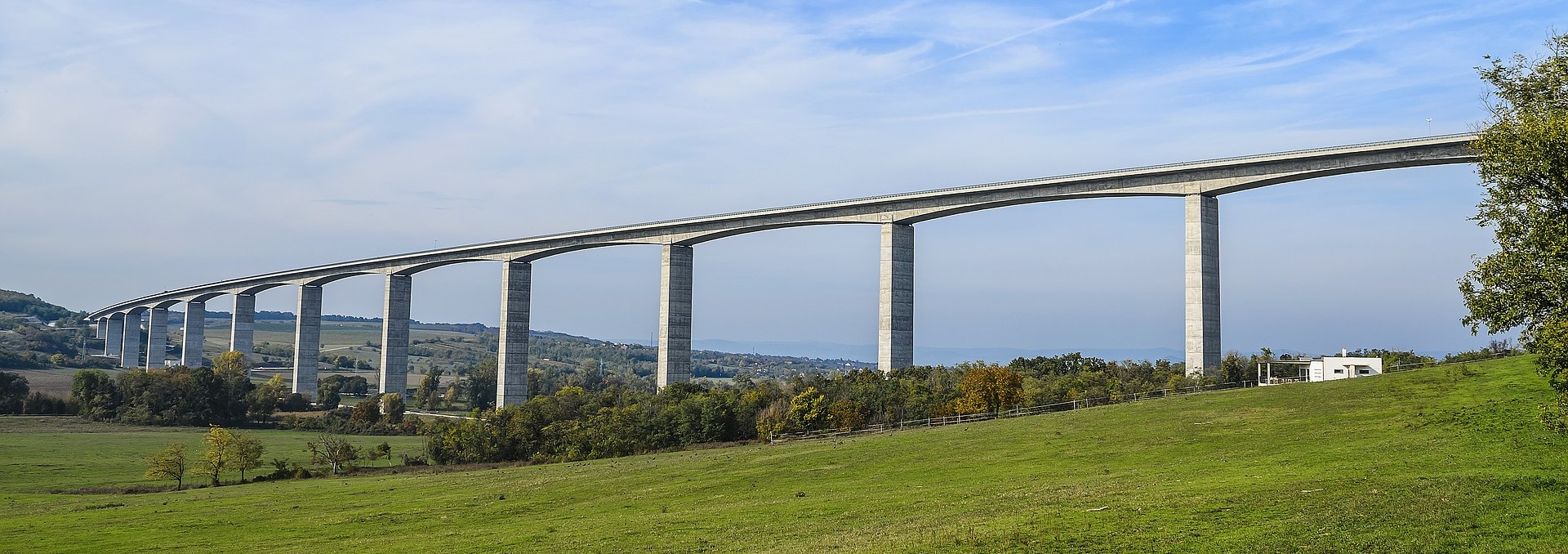
Development of new infrastructure, including new road bypasses or train lines such as HS2, often has some interaction with, and implications for, the floodplain. Bridges over rivers may constrict the flow at certain river stages. Embankments may interrupt normal flood extents increasing flood depths at certain locations. Whilst viaducts seek to minimize the interaction between the floodplain and roads and rail, there will always be some associated loss in flood storage and change in the overland flow due to the piers. A particular infrastructure scheme may alter all components of the source-pathway-receptor model (SPR). For example, it may increase surface run-off providing a new or increased source of flooding and it may alter the flood pathways; both of which may lead to a new receptor of potential flooding. Of course, the opposite is true and a proposed scheme may actually reduce the risk of flooding to a particular receptor. However, a reduction in flood extent is only beneficial if it does not increase flood depths in other areas particularly if this affects businesses, property or other critical infrastructure. In any case, it is essential to carry out a flood risk assessment (FRA) to analyse any change in flood risk associated with the scheme.
Hydraulic modelling is a useful tool to investigate any changes in flood regime caused by new infrastructure. River modelling using 1D/2D models such as Flood Modeller can be used to simulate the current flood extents for a given return period hydrograph as a baseline. Proposed developments can then be included in the model to see how they affect the extent and areas that flood and take into account increased precipitation and peak flows due to climate change. Further uses of the model include testing the efficacy of flood mitigation measures that seek to reduce flood risk to current receptors or to the actual scheme itself (e.g. raised tracks or replacing lost flood storage).
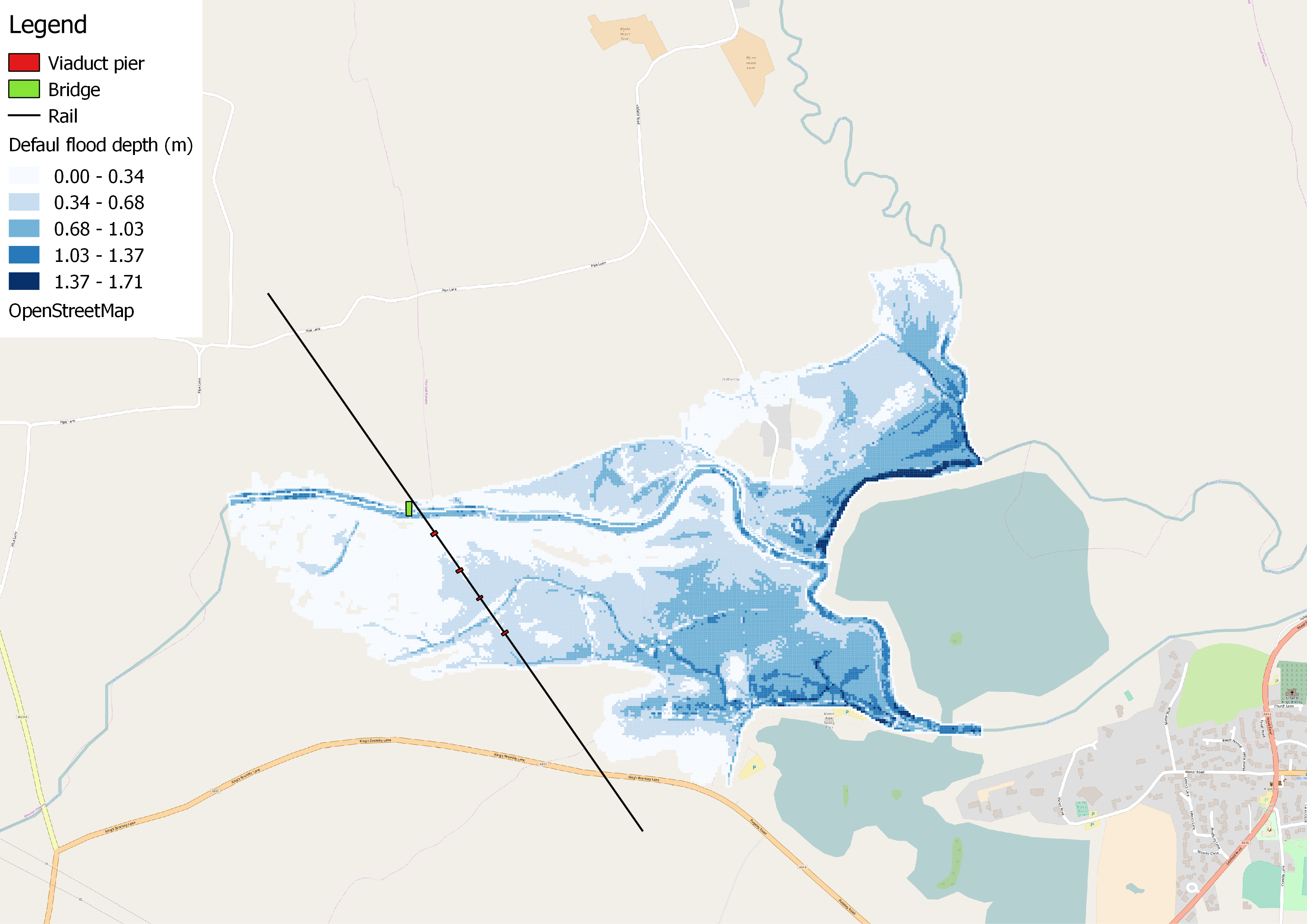
In the following sensitivity study, a design hydrograph is created that generates significant flooding either side of the River Trent between Pipe Ridware and Kings Bromley. Flood Modeller (formerly ISIS) was used to simulate the 1D channel flow with river cross-sections take from the Environment Agency's LIDAR composite digital terrain model (DTM). In the absence of survey data, this gives a reasonable representation of the channel shape and slope. However, the true channel depth and capacity is under estimated and a proper study should include a basic survey. In this instance, a Python script was used to smooth the channel and increase the channel depth slightly. However, the sensitivity of the results to this procedure was not examined. The out of bank floodplain inundation was simulated using a 2D model linked to the 1D river model. The following image shows the flood extent due to the design hydrograph and a key showing components of a hypothetical infrastructure scheme that includes a bridge and a viaduct with piers in the region of the current flood extent.
In the first sensitivity test, a bridge is included in the 1D river model to simulate the effect on the channel flow and subsequent flooding. Bridges constrict the river flow and increase the upstream water levels. Flood Modeller offers two methods for modelling bridges (read more here).
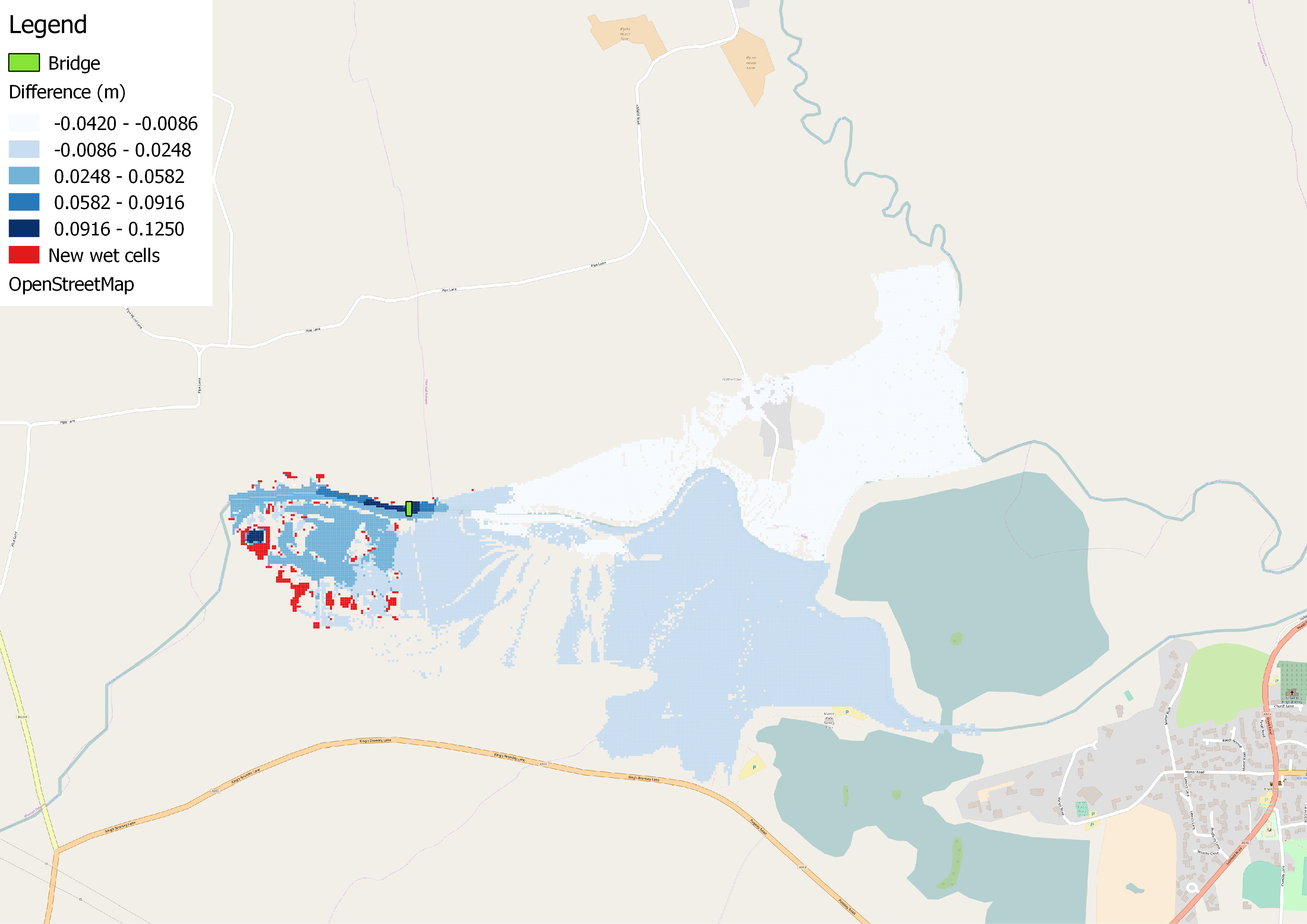
The image above shows the change in flood extent/depth due to the bridge. It can be seen that upstream of the bridge there are some increases in flood depths by up to 13 cm. The red areas also show that areas that were not flooded before are now flooded due to the presence of the bridge.
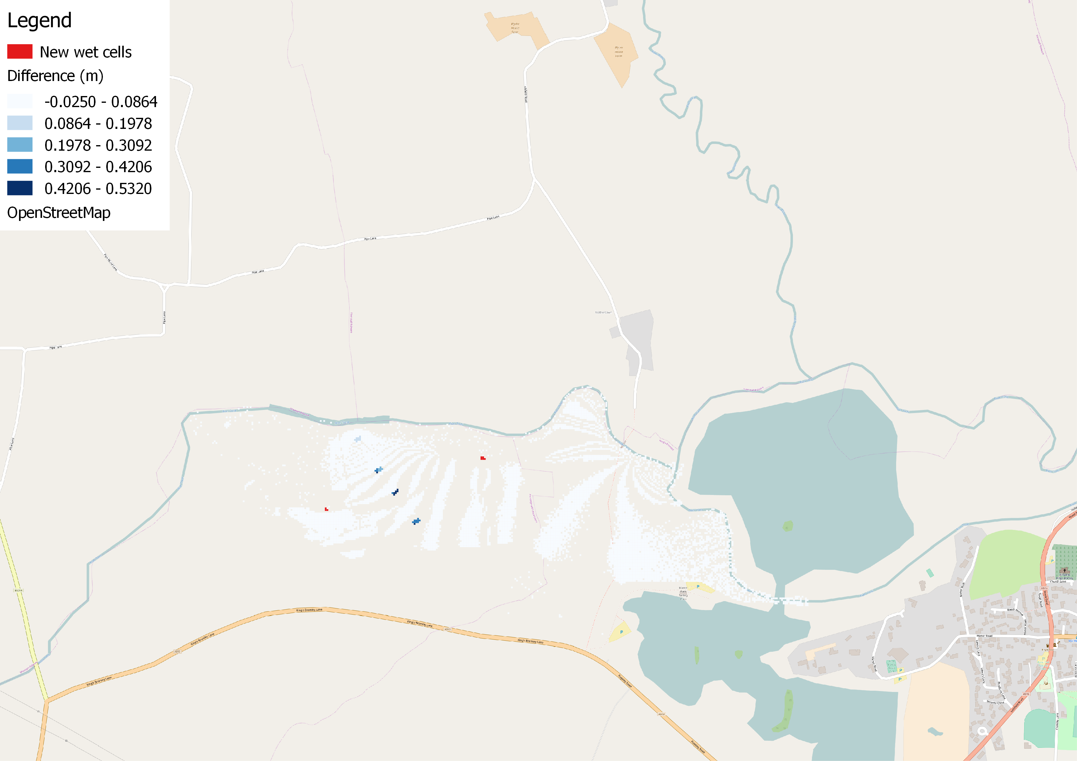
The image above shows the change in flood extent/depth due to the viaduct piers. It can be seen that the viaduct has little impact on the flood extent with a small number of newly flooded areas and an increase in flood depths localised to the piers due to pooling of the water.
Hydraulic modelling is useful for investigating the impact of infrastructure projects on rivers and floodplains, both now and in the future. After the initial time-cost associated with setting up the model, different structures and flood mitigation strategies can be implemented in the model reasonably quickly to examine their impact. This makes modelling a powerful tool for aiding flood risk assessments.
Mesh building and visualization
Tuesday, 30th May 2017
This blog was first published as a Linkedin article (see here) but is republished here.
This article relates to the first part of a three part video series on developing a coastal model. The first video (below) gives an overview on developing a computational mesh and this article aims to go into more detail about some of the tools and techniques used.
The video features various tools that I am developing at JM Coastal to make the whole process of developing a model and visualizing the output easier. I have used Django, a web development framework written in Python, to develop the tools. This means that the tools and model runs can be run on a local or remote server, provided the dependencies are installed at that location. As the video series will feature Telemac to run the coastal model, using Django is advantageous. This is because Telemac has a full suite of Python tools for parsing and manipulating the binary geometry and results files and managing the model runs thanks to the developers such as Sebastien Bourban.
The first task in mesh building to extract the coastlines in the desired domain. The coast line extractor tool featured in the video uses a JavaScript library for displaying and manipulating maps (OpenLayers) for the front end user interface. The user extracts the desired coastal line by drawing a polygon and the coastline is then extracted from a GSHHG global shape file from NOAA on the server side (using the Python GDAL bindings) for the user to download.
The mesh is generated using Blue Kenue. This is fantastic open source software for developing meshes, initial conditions, boundary conditions and visualizing results for hydrodynamic models in Telemac. The software can fit a triangular finite element mesh to a particular domain geometry with a resolution specified by the user or based on the underlying bathymetry. The bathymetry featured in the video comes from the EMODnet bathymetry database.
The bathymetry can be visualized in 3D in a web browser using threejs a JavaScript library that facilitates displaying 3D graphics using WebGL. The bathymetry is combined with a DTM and satellite imagery from EarthExplorer provided by USGS to create the 3D model. The terrain viewer featured in the video can be used to view 3D visualizations in your browser. There is a basic demo version of this application here.
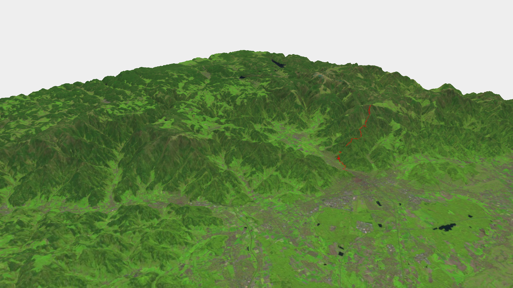
The example above is a 3D visualization of the Black Forest in Germany with a red line showing a GPS track of a hike from Freiburg to the top of Shauinsland, a nearby mountain. If you are a Python user and are interested in visualizing tracks from your GPS or applications such as Strava in Google Earth you can clone a gpx file parser I wrote (https://github.com/johnmaskell/gps_tools.git). The tool is useful for visualizing GPS surveys of coasts and rivers, such as dike inspections. It is worth noting that GIS software such as QGIS will also read gpx files from GPS.
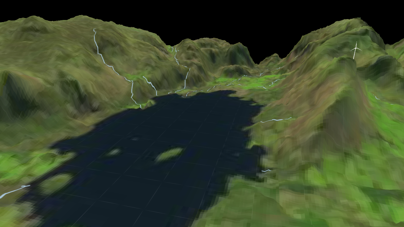
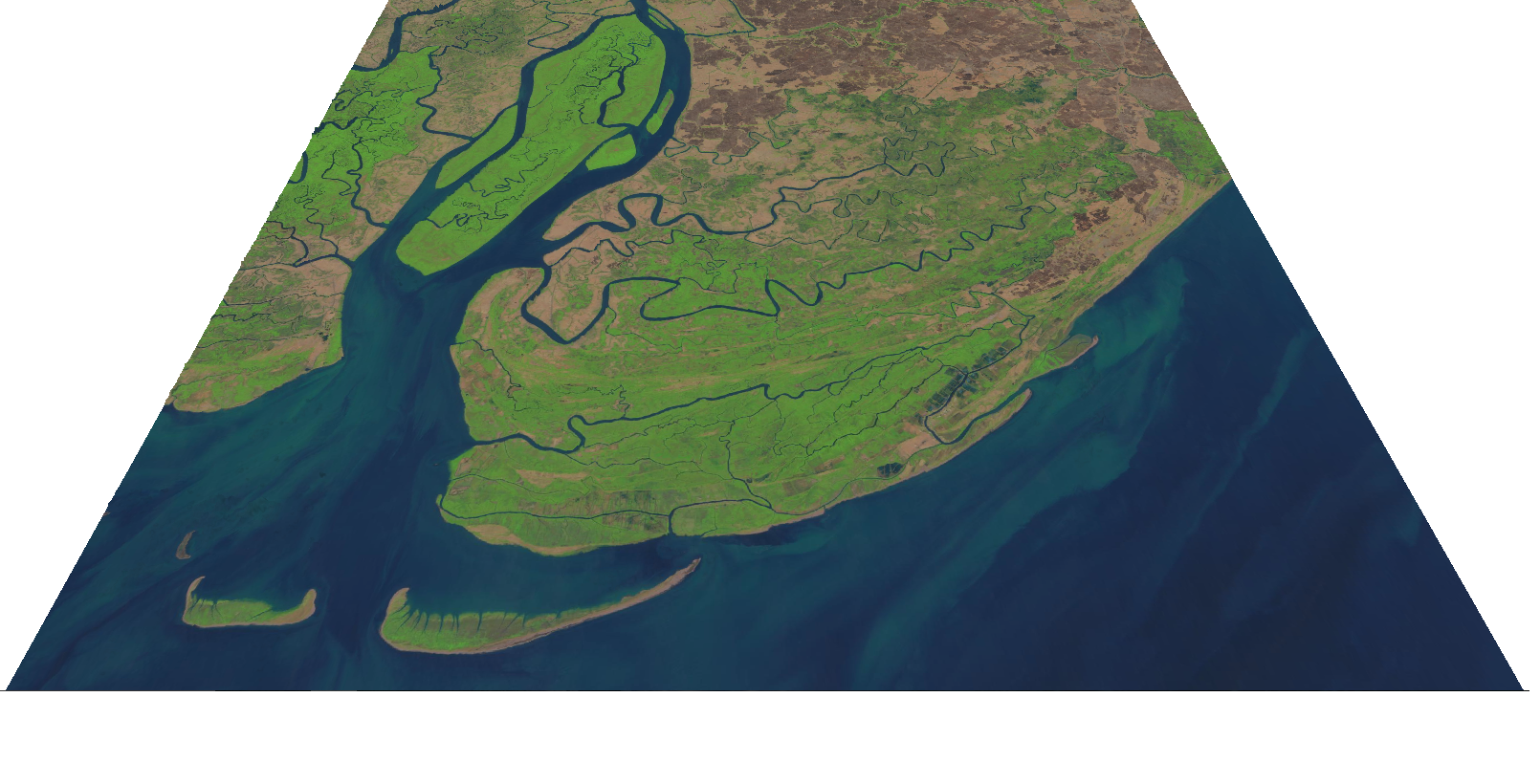
3D models in other formats (e.g. Collada) can be included for buildings or structures such as the wind turbine shown above. In low-lying regions such as the Ayeyarwady Delta region in Myanmar (shown below), relatively low resolution DTMs derived from satellites may appear spikey as the noise is relatively large in relation to the gradients in the relief.
The 3D terrain viewer will be further developed to visualize flood maps, beach profile changes and scour around structures in three dimensions. A great resource I came across for learning about visualization of geospatial data, is the Master Maps blog from Bjørn Sandvik.
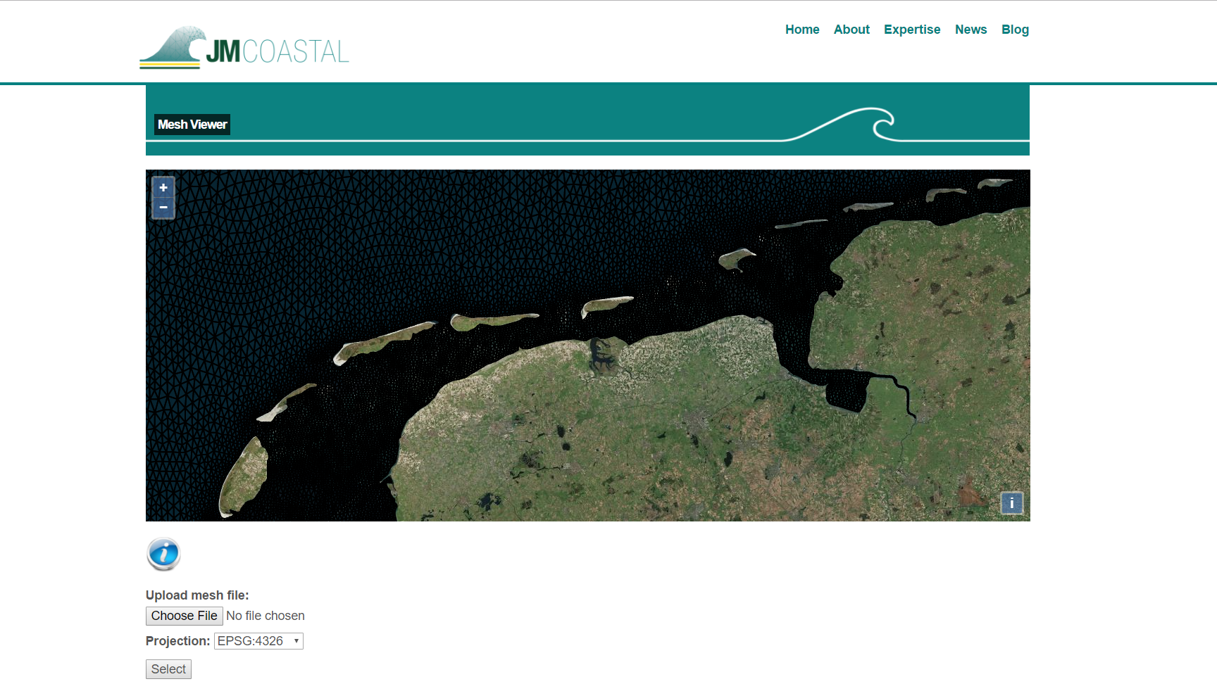
As with the coastline extractor tool, the mesh viewer tool (shown above), uses OpenLayers for the front end user interface where Python takes care of all the processing on the server side. The user can upload their mesh which is converted to kml. After the user has downloaded the kml file, they can drag and drop it onto the map in the browser or view it in Google Earth.
Look out for the next video in the series which will focus on carrying out a tidal simulation using the TPXO tidal database which is partially derived from satellite altimetry.
Running a tidal simulation
Tuesday, 04th July 2017
This blog was first published as a Linkedin article (see here) but is republished here.
This article relates to the second part of a three part video series on developing a coastal model. The first video covered setting up a computational mesh and some apps I developed to simplify some of the tasks involved. The second video (below) focuses on setting up and running a tidal simulation using the previously generated mesh.
The video features an app I developed that provides a user-friendly interface for setting up a tidal simulation in Telemac-2D using a global tidal constituent database. The app is developed in Python using the Django framework to connect the back end code to the user views. As a web-based application it can be used as a GUI on the user's computer or allow them to run a simulation on a local or remote server provided all the dependencies are installed at that location. The example here is only for a specific tidal simulation and does not provide all the options available in Telemac. A more complete version should be able to access the full Telemac dictionary in a database (e.g. MySQL) and a schema for rendering the web page with the correct forms based on the type of simulation the user would like to carry out.
Click on the image below to go to a demo version of the app.
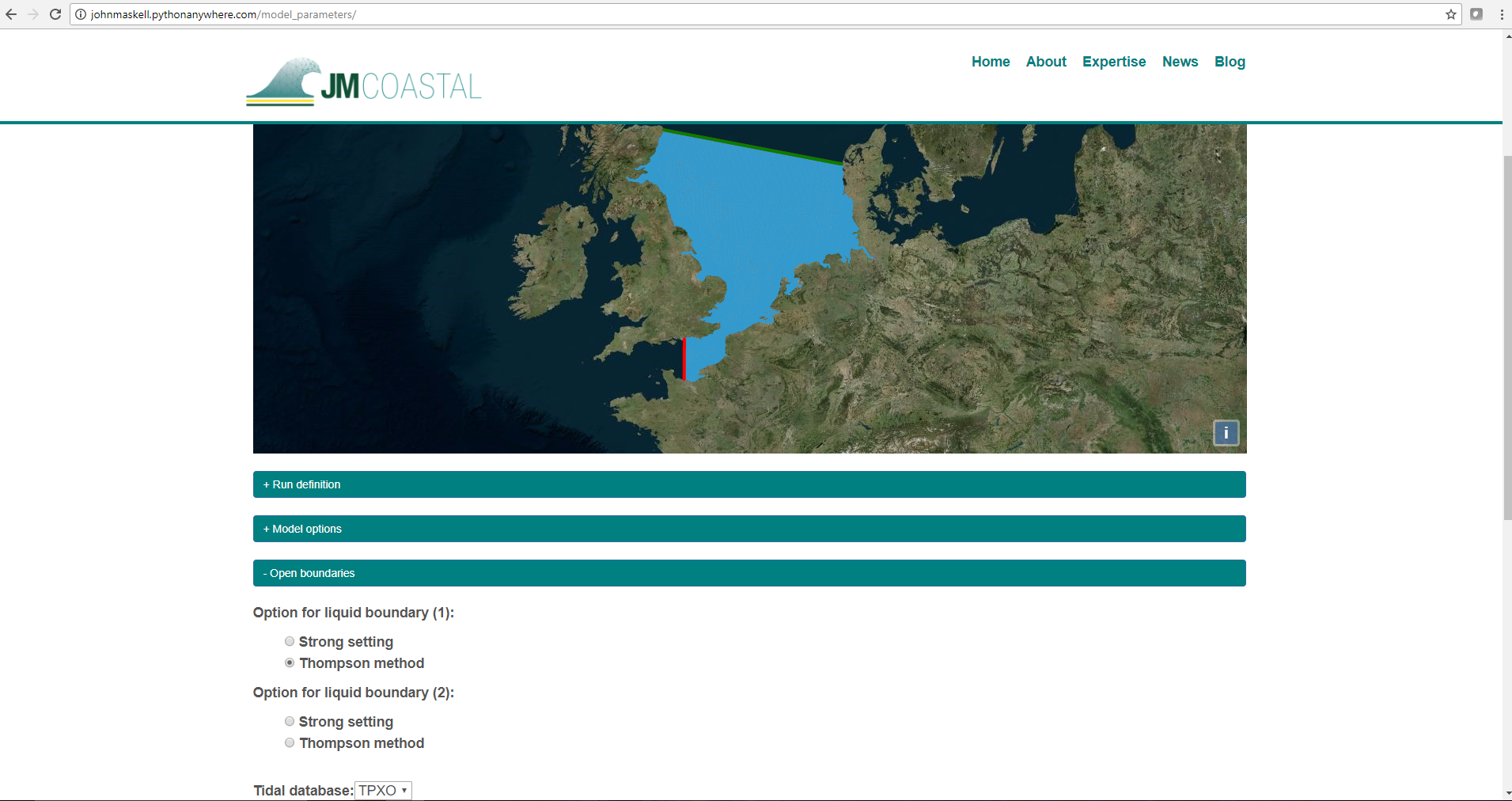
The user uploads a previously generated mesh which is parsed on the server side and reprojected to display in OpenLayers, a JavaScript library for displaying dynamic maps on web pages. The mesh is converted to GeoJSON to pass it from the server to the client side and added as a vector layer to the map. This is a nice way to visualize the mesh but very large meshes may make the map slow to load and unresponsive. The open boundaries are also passed as a GeoJSON and change from red to green once a valid open boundary option is chosen (see image above). The model set up is split into drop down menus to simplify the process and prevent the page from becoming too clustered. The example in the video shows the set up of a tidal simulation in the North Sea using the TPXO global tidal database.
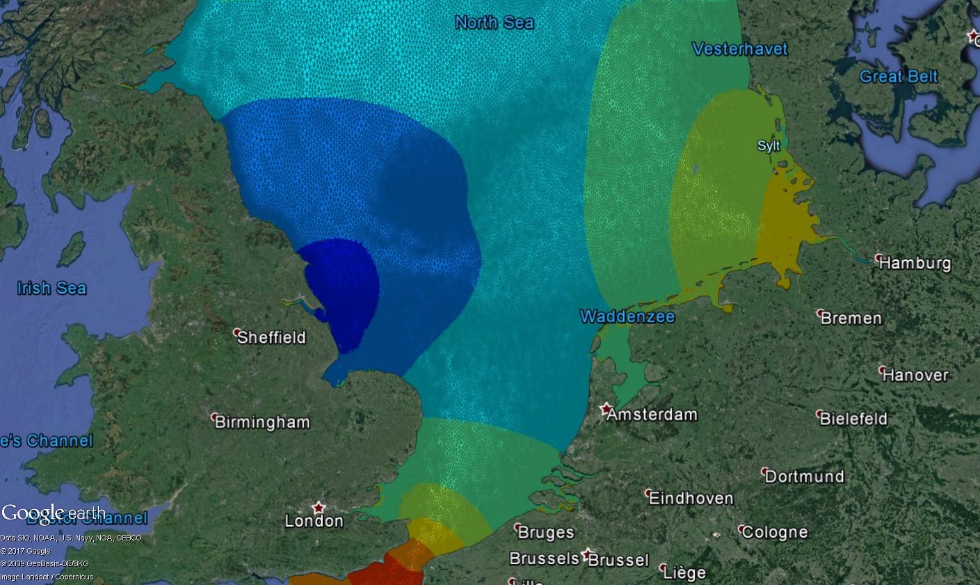
Read more about the North Sea tidal model here.
Additional options in the application allow the user to carry out an automatic calibration of the model and receive a text message when the model run is complete. For auto-calibration the user must upload a zip file containing tide gauge observations that fall within the model domain and cover the period of the simulation. Currently the application is set up to read UK tide gauge observations but should allow the user to enter the data format from other regions taking care to ensure the data has been cleaned. The current procedure looks at the RMSE in the high waters and tries to minimize the global error by altering the bed friction coefficient and the tidal range at the open boundaries. Future, options could include the wind drag coefficient for storm surge and waves and weighting factors for the observations to penalize observations in under resolved regions or outside the area of interest. The current procedure is sequential and therefore leads to long simulation times but this could be improved on a cluster by submitting at least two simulations at either end of a parameter range to try and close in on the best parameters.
Click on the image below to view the slideshow.
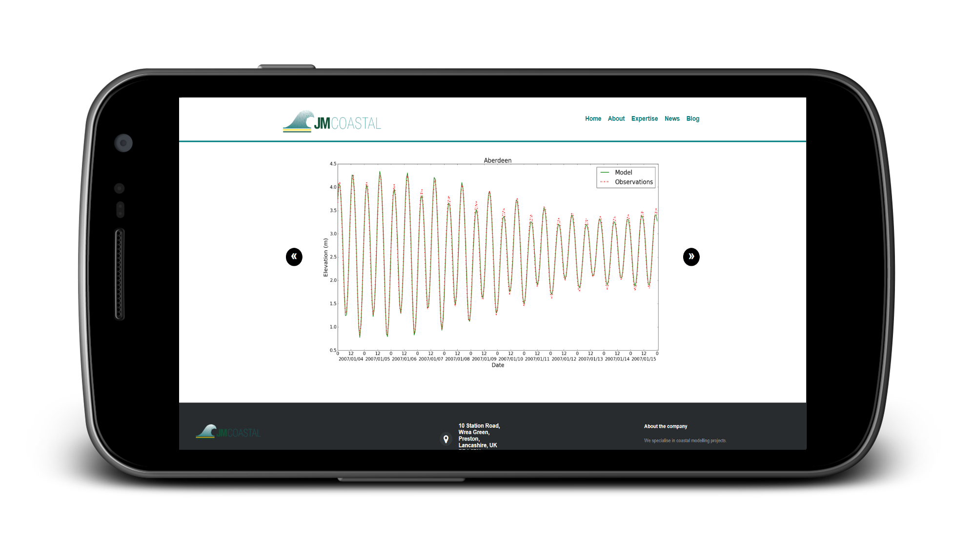
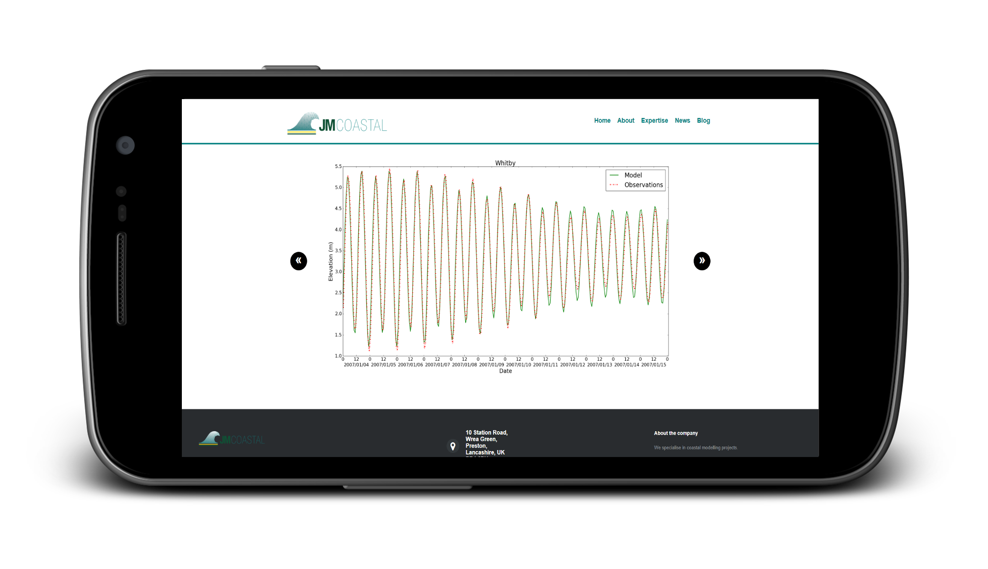
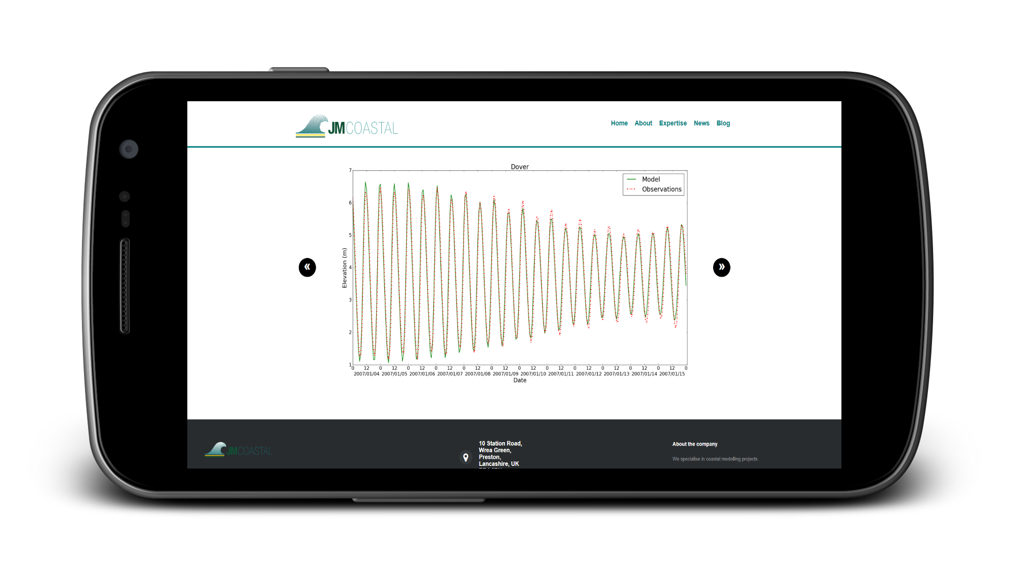
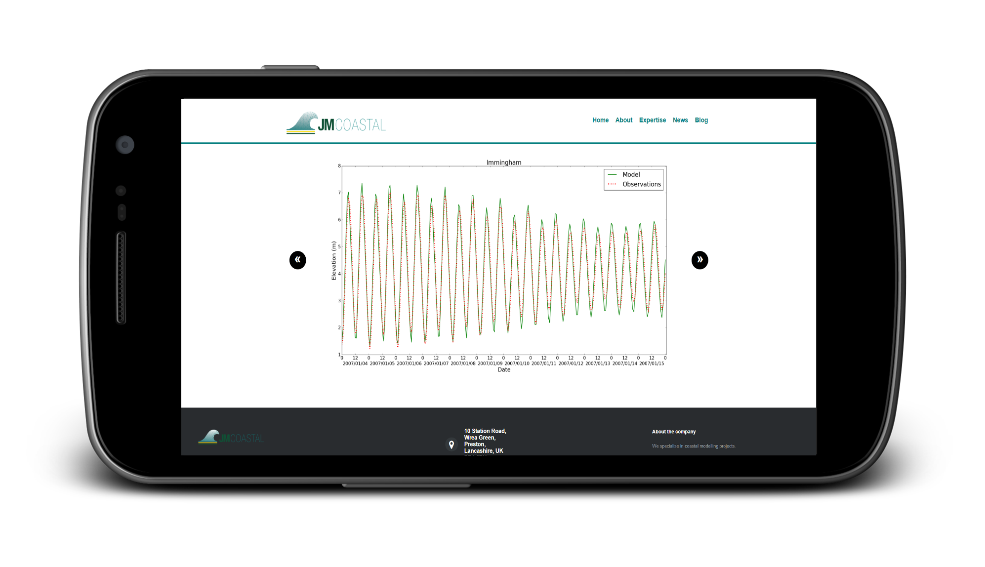
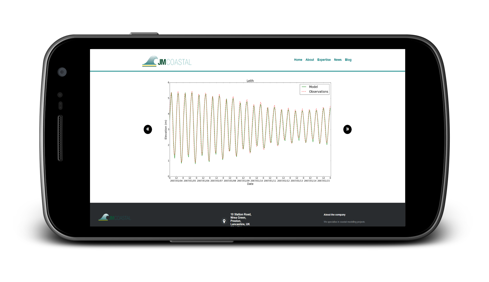
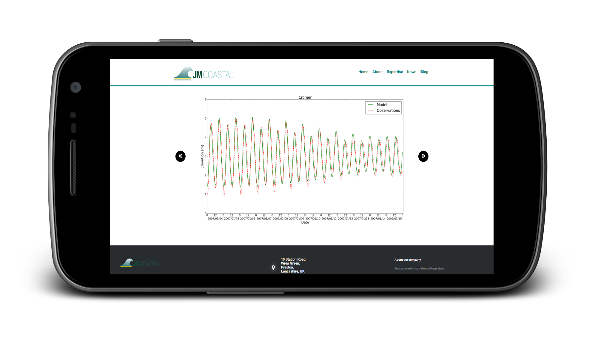
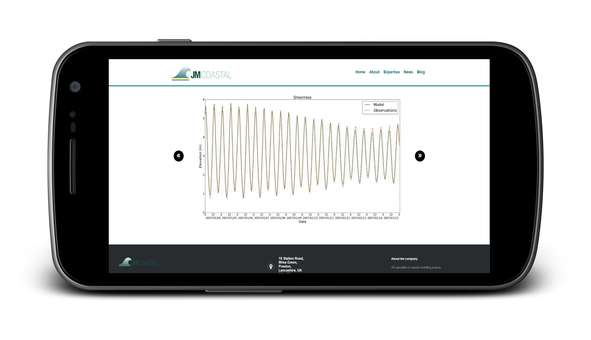
The user can also choose to have a text message sent to them after the model run is complete using the Twilio API. This can also contain a link to a web page with a slideshow of the observed vs. modelled time-series from the best auto-calibration run. This is probably of novelty value in this instance but could be useful in operational systems to distribute warnings and be combined with a mobile app that uses location services to warn users if their location falls within an area of predicted flooding.
Look out for the third and final video that will focus on extracting the model output and data visualization. Please get in touch if your organistaion would like a bespoke modelling platform developed for model testing and evaluation or operational purposes.
The need for speed - GPU power!
Monday, 13th November 2017
This blog was first published as a Linkedin article (see here) but is republished here.
Embarrassingly parallel (also called perfectly parallel or pleasingly parallel) - a computational workload or problem where little or no effort is needed to separate the problem into a number or parallel tasks (see Wikipedia). Flood simulations can be a good example of this. Once a grid is defined on which to calculate the shallow water equations, the solution cannot propagate more than one grid cell in a given time-step if the solution is bound by the CFL condition. In a regular grid the inter-cell fluxes are constrained to the ith cell and the four cells surrounding it. Therefore, at each time-step the exchange of mass and momentum at each cell can be computed in parallel, independently from the other cell groups. Simple right? Well there may be "little or no effort" in splitting the problem but the computational implementation may not be so simple and may take an embarrassingly long time! This is where the graphics processing unit (GPU) comes in.
GPUs
Originally designed to handle the rendering of computer graphics, GPUs are now used for a range or computational applications that can take advantage of their ability to accelerate certain applications. Whereas CPUs are optimized to carry out serial operations across one or multiple cores, GPUs are designed to carry out parallel computations across 1000s of cores. Artificial intelligence, robots, drones, self driving cars, molecular dynamics and flood modelling have all taken advantage of the speed up offered by GPUs.
Flood modelling
Users of flood models increasingly demand higher resolution. The availability of high resolution DTMs (<=1m) from Lidar allows users to simulate flooding at street/property level resolution. Users such as local planning authorities or the Cat Modelling/(re)insurance industry can take advantage of this increase in resolution to define flood risk zones, improve planning within them and in the latter case to put a more accurate price on risk or determine risk accumulations when it comes to potential flood losses. However, simulating large scale flood events is computationally demanding (e.g. the rainfall associated with Hurricane Harvey affected an area of nearly 75,000 km^2), particularly if you want to simulate numerous scenarios and/or the uncertainties around a given scenario. If you want to take advantage of the speed up offered by GPUs for flood modelling there is commercial software available (e.g. Tuflow, MIKE 21 or Flox-GPU). There are also opensource codes available such as from the Technical University of Munich who have a teaching code repository on GitHub. There are also numerous open source shallow water CPU codes (e.g. GeoClaw, FullSWOF or Nektar++) which you can adapt to run on a GPU and build your own code. I took advantage of FullSWOF and PyCuda to develop some code to speed up my own flood simulations. If you like Python, PyCuda is a great way to get into GPU programming through Cuda (NVIDIAs programming interface to their GPUs). Python can take care of all the input/output with the array handling capabilities of Numpy and the PyCuda library can be used to execute the GPU kernels (C++) within the same code. After an initial learning curve you can expect huge speed ups with little or no optimization. A good way to learn about parallel computing with libraries such as PyCuda is to attend one of the great free courses from PRACE. The training course "Parallel and GPU programming in Python" is coming up soon in Amsterdam (6th-7th December '17) for those who are interested. Some notes from a previous course can be found here.
Even with small computational grids the speed up is significant. The dam break experiment (see above) described in Ying et al (~800 grid cells) takes 25 seconds on my laptops CPU (Intel Core i7-5500U CPU @ 2.40GHz) using an adaptive grid and 0.035 seconds on the laptops GPU (Nvidia GeForce GTX 850m) with a fixed grid. The classic Malpasset Dam break simulation (see GIF above) takes 500 seconds for 373,205 grid cells (12 m resolution). I would have given a comparison to running this test case on my CPU but I gave up as it was taking so long! The DTM and initial conditions for the test case can be downloaded here.
The Telemac2D Malpasset Dam break case included in the examples (visualisation above) also takes about 500 seconds on the CPU with 104,000 computational cells. However, the main developers do report a time of 85 seconds when run in parallel on 8 CPU processors. It should be noted that the examples given here are not stringent comparisons as the hardware and solutions differ and are more to give an idea about the type of speed up that can be achieved with little or no optimizations.
Further applications
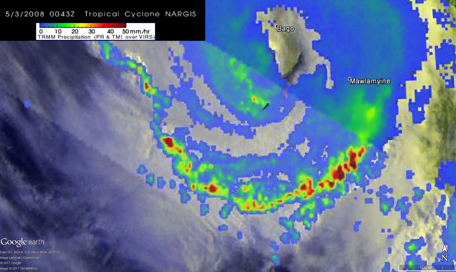
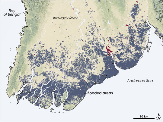
It is not all about dam breaks! The accelerated solutions can be applied to storm surges, tsunamis, river floods, rainfall run-off and pluvial events. To develop the application further I will generate a simulation of Cyclone Nargis that had devastating consequences in Myanmar. Due to the low lying land, significant storm surge and heavy rainfall (see image above - Hal Pierce, SSAI/NASA GSFC) a very large area was flooded (see image below - NASA/Robert Simmon).
A combined solution to the storm surge, rainfall fall run-off and accumulation and river flooding can take advantage of GPU acceleration to simulate the flood extents in a way that is computationally viable and allows sensitivity tests and uncertainty to be investigated.
For further articles and posts follow JM Coastal on LinkedIn.
Modelling Coastal Flood Risk - an e-learning course
Tuesday, 23rd April 2018
This blog was first published as a Linkedin article (see here) but is republished here.
Currently, 40% of the world’s population live within 100 kilometres of the coast. As population density, economic activity and development of new infrastructure continues to increase, our exposure to the risk of coastal flooding also increases. The risk of flooding is also likely to change in a future climate. Factors such as sea level rise, land subsidence and coastal erosion will increase the risk of coastal flooding even if the frequency of events that cause coastal flooding (e.g. tropical and extratropical cyclones) were to remain the same. Whilst it remains uncertain whether the frequency of extreme events, such as tropical cyclones, is likely to increase, it is likely that they will become more intense. Therefore, it is important that we try to gain a quantifiable understanding of coastal flood risk to aid or restrict coastal development, mitigate the risk with coastal defence schemes and make informed, evidence-based planning decisions. Coastal flood risk studies can be used to quantify the probability of the main drivers of coastal flood risk. Used in combination with numerical modelling studies to investigate potential consequences, it is possible to map areas at risk from potential flooding and aid mitigation plans.
What are we developing?
https://www.linkedin.com/pulse/modelling-coastal-flood-risk-john-maskell/At JM Coastal, we are developing an e-learning course that will teach the user to carry out a full coastal flood risk study using the available data. The course will have a theoretical component but with a strong emphasis on practical application. The user will gain some background knowledge in each component, a complete walkthrough the implementation of each component and be left at the end with a complete set of tools and open source software to use in further studies. Also, by gaining skills in coding languages such a Python and GIS software such as QGIS, the user could gain transferable skills in in demand topics such as data analysis and visualisation.
Why are we developing this course?
The course will address a knowledge gap in quantifying the risk of a coastal flooding due to the joint probability of the main drivers of risk, and propagating this through numerical modelling studies. Published standards on model methodology and quality will also increase the need for knowledge in all aspects of quantifying coastal flood risk to meet new requirements. We also aim to make such studies more accessible by giving an insight into the specialist components involved, and by providing the user with open source software.

How will the course work?
E-learning is a rapidly growing field of educational technology. It breaks down many of the barriers of traditional training and education and allows the user to learn from any location, at their own pace and in a cost-effective way. The Modelling Coastal Flood Risk course will be hosted on a specialist online learning management system (LMS). This will allow the user to access a range of audio and visual materials, gain access to the tools and software required and track their progress all in one place. The user will also benefit from a support forum to ask questions and overcome any issues that arise. The course will come at a fixed subscription cost which will then allow the learner to have access to all the course and the materials for an unlimited amount of time.
You can view or download the full course notes here. If you would like more information and want to stay up to date with the course release date please add you email to the mailing list here or in the form below.